Continuing Date Pattern in Google Sheets

This tutorial about utilizing Google Sheets date functions divided into three subcategories for easy explanation – Simple Date Functions, Standard Date Functions, and Advanced Date Functions.

I have spent lots of my time writing tutorials related to Google Sheets' advanced functions, charts and other important aspects related to Google Sheets.

As a result, you can see plenty of tutorials related to Google Sheets on this Site. So what's the point?

The thing is that I intentionally opted out of writing some of the commonly being used Google Sheets functions which I thought users might know. The Google Sheets Date functions are one among them.

In order to make Info Inspired a complete reference source for Google Sheets users, I am filling that void space with the so-called 'missing' functions.

So here we are. Let us begin with how to utilize Google Sheets Date functions.

Simple Google Sheets Date Functions

Google Sheets TODAY Function

How to use the TODAY function in Google Sheets?

When you want to return the current date on a cell use this function. Remember, the date thus inserted will auto update.

          =TODAY()        

Google Sheets DAY Function

How to use the DAY function in Google Sheets?

Syntax:

          =DAY(date)        

Purpose: The DAY function in Google Sheets returns the day from a given date.

Argument:

date – The date from which to extract the day.

Example to Sheets DAY Function.

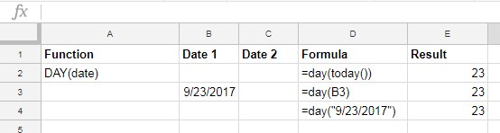
In cell E2, the formula returns the current day. As you can see, in cell E3, the formula returns the day from the given date in cell B3. Finally, the formula in cell E4 returns the day from a given date inside the formula.

NOW Function in Google Sheets

How to use the NOW function in Google Sheets?

The NOW Google Sheets function is similar to the TODAY function. The TODAY function returns only the current date. But the NOW function returns the DateTime. Needless to say, both are volatile.

          =NOW()        

Google Sheets MONTH Function

How to use the MONTH function in Google Sheets?

Syntax:

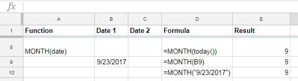
          =MONTH(date)        

Purpose: Google Sheets MONTH function returns the month (in numerical format) from a given date.

Arguments:

date – The particular date from which to extract the month.

Example to the MONTH function:

Google Sheets YEAR Function

How to use the YEAR function in Google Sheets?

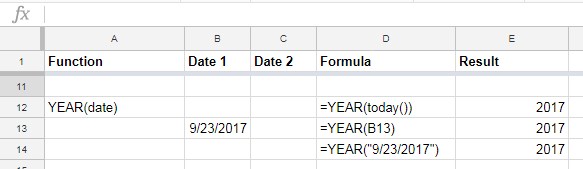
          =YEAR(date)        

Purpose: Google Sheets YEAR function returns the year (in numerical format) from a specific date.

Arguments:

date – It's the date from which to extract the year.

See some example formulas to the YEAR function in Docs Sheets.

Standard Google Sheets Date Functions

As I have mentioned above, the above categorizations of Google Sheets Date functions are simply for explanation purpose. There is no such categorization in the real sense.

Let us begin with Standard Google Sheets Date functions.

Google Sheets DATE Function

How to use the DATE function in Google Sheets?

Syntax:

          =DATE(year, month, day)        

Purpose: Use Google Sheets DATE function to convert a provided year, month, and day into a date.

Arguments:

year – It's the year component of the date.

month – It's the month component of the date.

day – It's the day component of the date.

Example to the DATE function in Sheets.

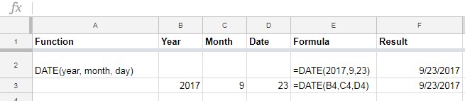
Sometimes we keep the year, month and date in separate columns like in cell B3, C3, and D3 respectively. So this function is to return the date from such entry.

DATEVALUE Function in Google Sheets

How to use Google Sheets DATEVALUE function?

Syntax:

          =DATEVALUE(date_string)        

This is one of the very useful date functions in Google Sheets.

Purpose: The Datevalue function converts a date stored as text to a serial number that Google Sheets recognizes as a date. You can later utilize theto_date() function to convert back that serial number to date.

Arguments:

date_string – It's the string representing the date.

Usage Notes:

When you use a string inside the DATEVALUE formula you can apply different date formats. See the below example screenshot where I've applied different date formats inside the formula (except row # 10).

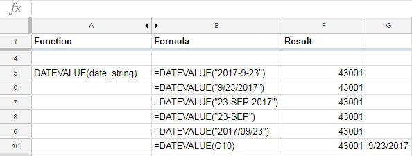
But when you use DATEVALUE function to refer to a cell (refer the formula in cell E10), that date should be entered as per the standard date format set on your spreadsheet.

You can check this by entering a date in any cell (cell G10 as per my example). If the entered value is a date, it would normally get aligned to the right.

Now format that date (in cell G10) to text from the menu Format > Number > Text. It won't affect the DATEVALUE formula output.

DAYS Function in Google Doc Sheets

How to use the DAYS function in Google Sheets?

Syntax:

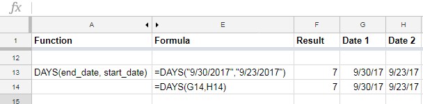
          =DAYS(end_date, start_date)        

Formula examples and purpose:

You can utilize this google sheets date function to find the date difference in number. That means the number of days between two given dates.

Normally the start date will be a past date and the end date will be a future date. If you use these dates on the reverse, the formula will return a negative number.

          =DAYS("26/03/2019","26/04/2019")        

Result: -34

Google Sheets DAYS360 Function

How to use the DAYS360 function in Google Sheets?

Syntax:

          DAYS360(start_date, end_date, [method])        

Purpose: Use to calculate the difference between two days based on the 360-day year.

Arguments:

start_date

end_date

method – Day count method indicator.

I have seen Google Sheets users wrongly using DAYS360 function instead of the DAYS function. If you use DAYS360 without knowing the usage, you will get the wrong output.

Suppose if you just want to find the difference of days between two dates, use the function DAYS or DATEDIF.

Formula Example to the DAYS360 function in Sheets:

          =DAYS360("30/03/2018", "31/03/2018", 1)        

The above formula returns 0, not 1. Why?

Here at the end of the formula, I've used the day count indicator 1. It's the European method where any start date or end date that falls on the 31st of a month (see the above dates in the formula), has its day of month changed to 30.

If you leave the method blank, the formula follows the US method in that if a start date is the last day of a month, the day of the month of start date is changed to 30 for the purposes of the calculation.

In concise you can use the DAYS360 function in financial interest calculations.

Google Sheets Advanced Date Functions

Now let us see how to utilize some advanced date functions in Google Sheets. These functions are also simple but as a beginner, some of you may find a tough time with it. That is why I put it under advanced date functions. Here we go!

EDATE Function in Google Doc Sheets

How to use the EDATE function in Google Sheets?

A very useful date function in Google Sheets which will come in handy in date related conditional formatting.

Syntax:

          =EDATE(start_date, months)        

Arguments:

start_date

months – The number of months before (-ve) or after (+ve) the 'start_date' to calculate.

Purpose:

Use Google Sheets EDATE date function to return a date after or before a given date that based on the number of months as input.

For example, you can get a date after six months of a given date or 5 months back of a given date. That month's part is important. See the formulas below.

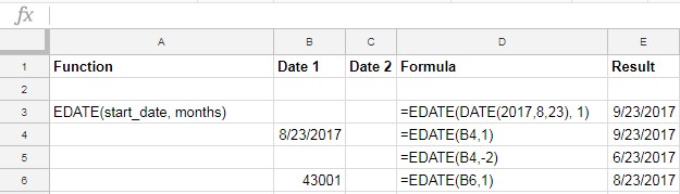
This function also accepts date value, see the DATEVALUE function, which is already detailed above.

Google Sheets ISOWEEKNUM Function

How to use the ISOWEEKNUM function in Google Sheets?

Syntax:

          =ISOWEEKNUM(date)        

To understand this Google Sheets function, you should first know what is ISO Week. This Wiki article will be helpful to you to know about the ISO Week in detail.

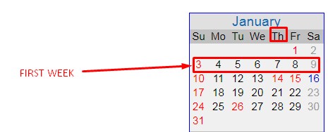
ISO Week in a Nutshell:

• The ISOWEEKNUM function follows the ISO 8601 date and time standard.
• In this standard weeks begin on Monday and end on Sunday.
• As per this standard, Week 1 of the year is the week that containing the first Thursday of the year.

See the below image.

Formula examples to the ISOWEEKNUM function in Sheets:

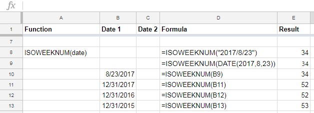
The above ISOWEEKNUM formulas return the numbers of the ISO weeks of the year where the provided date falls.

NETWORKDAYS Function in Google Doc Sheets

How to use the NETWORKDAYS function in Google Sheets?

Syntax:

          =NETWORKDAYS(start_date, end_date, [holidays])        

You can utilize NETWORKDAYS function to get the number of networking days between two given dates. Then what is networking days?

Normally networking days are the total number of days excluding weekends. Weekends here means Saturday and Sunday. If you want to change the weekends there is another function, that follows after this.

Optionally you can exclude holidays also. Examples are always the best method to learn.

See how I have excluded the US Federal holidays in 2019 in the net working day count.

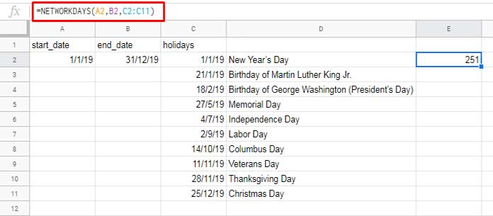
If any of the provided holidays falls on weekends, it won't get deducted twice.

To cut short this tutorial as well as to make things simple, I've opted out the string method this time. The same will be followed in the coming examples.

Google Sheets NETWORKDAYS.INTL Function

This is one of my favorite Google Sheets Date functions. You will also agree to it once you learn it.

How to use the NETWORKDAYS.INTL function in Google Sheets?

Syntax:

          =NETWORKDAYS.INTL(start_date, end_date, [weekend], [holidays])        

This function is superior to NETWORKDAYS. How?

The NETWORKDAYS.INTL is almost the same as the NETWORKDAYS function.The only difference is, the former function allows you to specify the weekends.

This is useful when in some countries like the middle east, Friday and Saturday are considered as weekends.

To use NETWORKDAYS.INTL function, you should know the weekend numbers.

What are the Weekend Numbers in Google Sheets?

If weekends are 2 days;

• Saturday, Sunday – Weekend Number is 1.
• Sunday, Monday – Weekend Number is 2.
• Monday, Tuesday – Weekend Number is 3.
• Tuesday, Wednesday – Weekend Number is 4.
• Wednesday, Thursday – Weekend Number is 5.
• Thursday, Friday – Weekend Number is 6.
• Friday, Saturday – Weekend Number is 7.

If weekend is 1 day only;

• Sunday only – Weekend Number is 11.
• Monday only – Weekend Number is 12.
• Tuesday only – Weekend Number is 13.
• Wednesday only – Weekend Number is 14.
• Thursday only – Weekend Number is 15.
• Friday only – Weekend Number is 16.
• Saturday only – Weekend Number is 17.

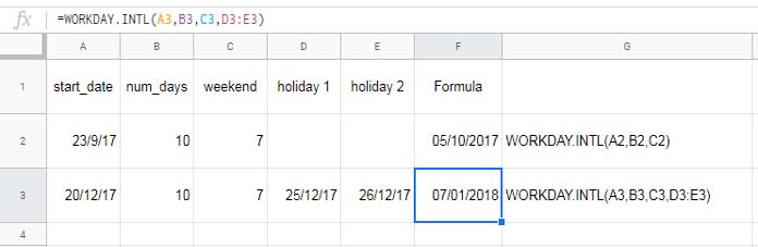
Now let us go through two example formulas.

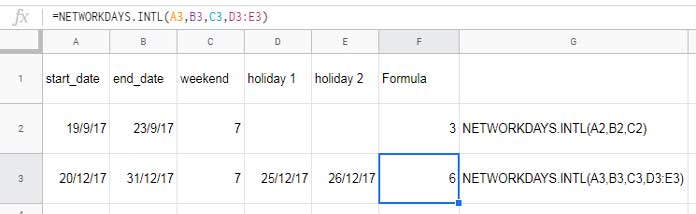
To understand the above NETWORKDAYS.INTL formula in cell F3, see the below calendar.

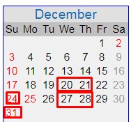
In the formula, what I want is to find the working days during the period from 20/12/2017 to 31/12/2017. The holidays are on 25/12/2017 and 26/12/2017.

I have used the weekend number 7 in the formula, which denotes weekends as Friday and Saturday.

So the remaining days I've marked in the above calendar and when you count it, you will get the number 6 and that is the result of the formula.

WORKDAY Function in Google Sheets

How to use the WORKDAY function in Google Sheets?

Syntax:

          =WORKDAY(start_date, num_days, [holidays])        

The WORKDAY function has lots of similarities with the NETWORKDAYS function which I have already detailed above.

We utilize NETWORKDAY to find the number of working days between two given dates excluding weekends and holidays.

Here in WORKDAY, we can find a date after a given number of working days.

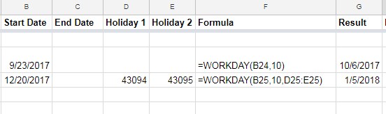
Suppose today is 01/01/2017. We can use the WORKDAY function to find a date after 90 working days. Working days means days excluding weekends and holidays.

First please learn above NETWORKDAYS function then come back to WORKDAY function so that you can easily grasp.

Helpful Tips: Use negative number in the place of num_days to count backward.

Google Sheets WORKDAY.INTL Function

How to use the WORKDAY.INTL function in Google Sheets?

Syntax:

          =WORKDAY.INTL(start_date, num_days, [weekend], [holidays])        

All the Google sheets date functions ending with INTL are so special to me. Such Google Sheets date functions will be useful if you have employees deployed around the world. Because weekends as well as holidays may differ among countries.

The WORKDAY.INTL function is same as the WORKDAY function. But here the difference is, you can change the weekend days.

Please refer NETWORKDAY.INTL function and then the WORKDAY function above. Then come back to here.

You can use WORKDAY.INTL function to return date after giving input as the number of working days.

Suppose today is 01/01/2017. You want to find a future date after 180 working days. Additionally you want to exclude the weekends of your choice and your selected holidays. Then use WORKDAY.INTL function.

There are weekend codes or identification numbers that required in the function. Find it above under the function NETWORKDAYS.INTL.

Here in this example, I've used weekend number 7 which indicates Friday and Saturday as weekends. If you want to use Saturday and Sunday as weekend days, use weekend number 1.

YEARFRAC Function in Google Sheets

How to use the YEARFRAC function in Google Sheets?

Syntax:

          =YEARFRAC(start_date, end_date, [day_count_convention])        

YEARFRAC is yet another useful Google Sheets date function. Use this date function to return the number of years including fractional years between two given dates.

In the YEARFRAC formula, you can specify which day count conversion to be followed. There are four different day count conversions in Google Sheets.

What is day count conversion?

It is like how many days in a year to be considered. Whether it's 360 days as a year or 365 days or the actual number of days in a year as the year.

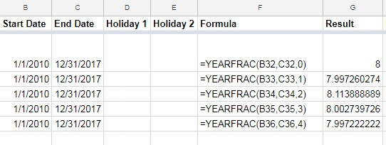
Day count conversion numbers.

• 0 indicates 30 days each month. That means 360 days in a year, i.e. 30/360.
• 1 indicates actual days between two specified days, i.e. actual/actual.
• 2 indicates the actual number of days between two specified days but assumes 360 day year, i.e. actual/360.
• 3 indicates the actual number of days between two specified days but assumes a 365 day year i.e. actual/365.
• 4 is similar to 0, this calculates based on a 30 day month and 360 day year but adjusts end-of-month dates according to European financial conventions, i.e. European 30/360.

Confused? Don't worry! I have included all the above count conversion numbers within the below formulas. Also, detailed information about the count conversion numbers can be found on this Wiki page.

Formula examples to the YEARFRAC function in Google Sheets.

DATEDIF Function in Google Sheets

How to use the DATEDIF function in Google Sheets?

Syntax:

          =DATEDIF(start_date, end_date, unit)        

DATEDIF is one of the very useful functions among the available Google Sheets date Functions. This is not DATED IF function. It is DATE DIF function. What's it?

This function will do the job of three functions. What are they? The DATEDIF function calculates the number of days, months, or years between two given dates with the help of unit abbreviation.

What is the "unit" in the syntax?

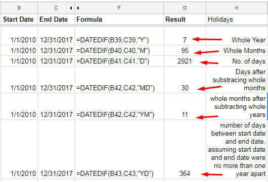
It's a text abbreviation for the unit of time. Where;

• "Y" stands for the number of whole years between a start date and end date.
• "M" stands for the number of whole months between a start date and end date.
• "D" stands for the number of days between a start date and end date.
• "MD" stands for the number of days between a start date and end date but after subtracting whole months.
• 'YM" stands for the number of whole months after subtracting whole years.
• "YD" stands for the number of days between a start date and end date, assuming start date and end date were no more than one year apart.

Example to the DATEDIF function in Docs Sheets:

Google Sheets WEEKDAY Function

How to use the WEEKDAY function in Google Sheets?

Syntax:

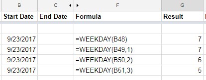
          =WEEKDAY(date, type)        

Purpose: The WEEKDAY function in Sheets returns a number representing the day of the week of the provided date.

First I will tell you what is the "type" in WEEKDAY date function.

Type is optional in the function. If omitted or put as 1, the day count will start from Sunday to Monday. In this case, the weekday number for Sunday would be 1 (Sunday 1, Monday 2, Tuesday 3, … Saturday 7).

If you put 2 then the counting will start from Monday to Sunday (Monday 1, Tuesday 2, Wednesday 3 … Sunday 7). See a few examples.

If you put 3 then the counting will start from Tuesday to Monday.

Google Sheets WEEKNUM Function

How to use the WEEKNUM function in Google Sheets?

Syntax:

          =WEEKNUM(date, [type]        

The WEEKNUM function returns a number representing the week of the year where the given date falls.

Similar to WEEKDAY function you can determine which day to consider as the week start day.

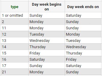
Note: The week containing January 1 will be numbered as week 1. This is applicable to type 1 to 17. In type 21, the week containing the first Thursday of the year is numbered as week 1.

Formula example to the WEEKNUM function in Sheets:

The formula in cell C2 which is dragged/copied down:

          =weeknum(A2,2)        

Formula in cell E2 which is also dragged/copied down:

          =weeknum(A2,21)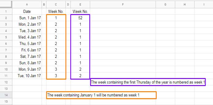        

In both the formula types (type 2 and 21), the day week begins on Monday and day week ends on Sunday.

Let us conclude this ultimate Google Sheets Date Functions tutorial. Now to the last function.

EOMONTH in Google Sheets

How to use the EOMONTH function in Google Sheets?

Syntax:

          =EOMONTH(start_date, months)        

This function simply returns the end of the month of a given date.

Suppose our date to be checked in cell C4 is 01/24/2017.

You can apply the formula below.

          =eomonth(C4,0)        

In this formula, "0" represents the current month. It will return the last date of the month, i.e., 01/31/2017.

If you change the value to "1", it will return the next month last date and so on. Enter the below formula on your Sheet and check the output.

          =eomonth(today(),-1)        

Conclusion

I don't want to drag this tutorial to anymore! Because I know already this tutorial got a bit lengthy.

I myself never thought these much time I would take to complete this tutorial. I took more than 10 hours at a stretch to complete this Google Sheets Date Functions tutorial! If you find it useful please share.

milesafearighted.blogspot.com

Source: https://infoinspired.com/google-docs/spreadsheet/google-sheets-date-functions-complete-guide/

Share this post